This episode is a live recording of the eighth session of #UnblindingResearch held in DREEAM 23rd October 2018. The group work has been removed for the sake of brevity.

This session of #UnblindingResearch looks at deciphering p values and confidence intervals and the factors behind healthcare outcomes and their measurement. Here are the slides for this session (p cubed of course), you can move between slides by clicking on the side of the picture or using the arrow keys.

Here is the #TakeVisually for this session:

p values

Imagine you’ve created a new beta blocker called Superlol which you want to be the most widely used anti-hypertensive in the world. You’d want to know how it compares to other beta blockers already used. Before testing you’d make a null hypothesis which would be something like “Superlol does not reduce patient’s blood pressure better than other beta blockers”.

During any study there would be false positives (subjects whose blood pressure is reduced due to chance not due to Superlol) and false negatives (subjects where there was a reduction but it was missed by the test). Too many false positives and our study would conclude that Superlol works when it doesn’t (falsely reject the null hypothesis). This is Type I error. Too many false negatives and our study would conclude that Superlol doesn’t work is does (falsely accept the null hypothesis). This is Type II error.

In the previous session we talked about significance and power. Significance (α) is how we reduce the chance of Type I error. In the previous session we went through how we decide what significance we want for our study and this impacts on our sample size. Significance is represented by a p value which is a decimal. The p value shows the chance that the observed result was due to chance alone. The gold standard is p<0.05 which means there is a less than 5% chance the result of the study was due to chance. If our study has p<0.05 and finds that Superlol reduced blood pressure in our subjects then we can call the effect significant. If we are only interested in whether Superlol is not inferior to other beta blockers then the significance is one tailed (all of the p value is allocated to that one direction). If we are interested if whether Superlol is not only non-inferior but also superior then the significance is two tailed (half of the p value is allocated to each direction).

Power (β) is about reducing Type II error. Again, this is decided at the beginning of our study and affects sample size. We know that there will be some false negatives and accept a certain amount. Power is again represented by a decimal, the gold standard being 0.8. This means that the study is powered so 80% of negatives found will be true negatives; no more than 20% will be false negatives. Therefore if we have a power of 0.8 and find that Superlol isn’t as good as other beta blockers then the study is powerful enough for us to conclude that that is the correct result.

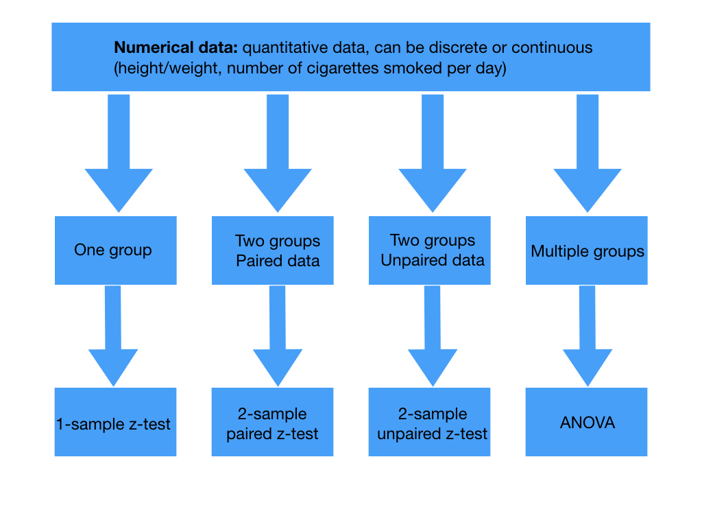
When calculating a p value we need a test statistic. This is a variable from the data we use to test our hypothesis. Picking the test statistic depends on the type of study and the data we’re collecting. Our data for our trial into Superlol would be called parametric as we would know the population distribution of blood pressure and our sample would be large enough. Depending on your trial then if your data is parametric there’s a choice of tests to calculate your test statistic:

Tests for the test statistic in numerical data. Paired data arises from the same individual at different points in time while unpaired data comes from separate individuals. T tests are used if the sample is small or if population standard deviations… — Tests for the test statistic in numerical data. Paired data arises from the same individual at different points in time while unpaired data comes from separate individuals. T tests are used if the sample is small or if population standard deviations are not known.

Tests for the test statistic in categorical data

It’s worth pointing out that if the population distribution is not known and sample size is too small then data is non-parametric so other tests are used:

Wilcoxon signed rank test (paired numerical data)
Wilcoxon rank sum test or the Mann Whitney U-test (unpaired numerical data)
Kruskal-Wallis test (non-parametric equivalent of analysis of variance (ANOVA))

Back to Superlol. Say we’re comparing the mean systolic blood pressure on Superlol to the mean systolic blood pressure on another beta blocker. Looking at the above tables as this would be comparing two groups of unpaired numerical data we’d use the two-sample unpaired t-test.

Say that this gives us a test statistic of 2. There are calculations which allow us to work out a p value from this test statistic. This gives us a p value of 0.0455 which would be considered statistically significant. If z = 1 then p = 0.3173 and it would not be considered statistically significant.

Confidence intervals

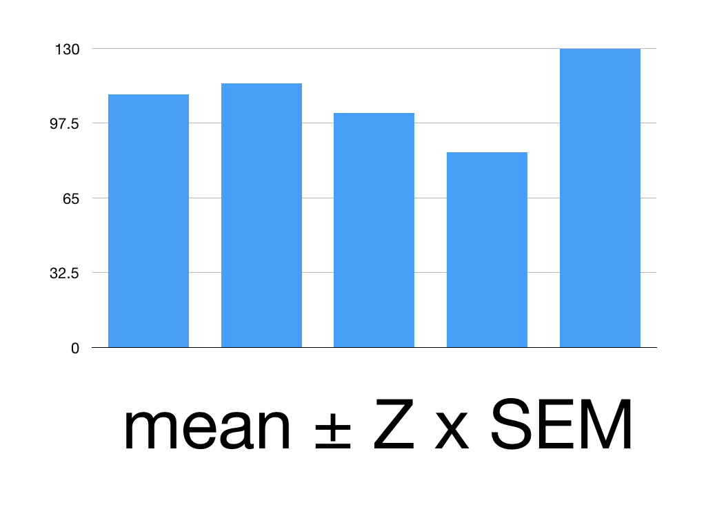
No treatment being studied is going to give the same results in each individual participant. Blood pressure varies over the course of a day and is affected by other variables such as mood, activity, body habitus and gender. So in studying Superlol our subjects will need to record their BP on many days for us to take a mean for each subject. You’ll see that each subject has a different mean BP.

This variability is known as the standard error of the mean (SEM). SEM can be estimated by dividing the standard deviation by the square root of the sample size. The smaller our SEM the more precise our data. SEM does not reflect accuracy.

Confidence intervals represent both the accuracy and the precision of an estimate. It is derived from the SEM but the idea is it allows us to picture the variation more easily. The interval is the range of values in which we can be confident the true value of our population parameter lies. That amount of confidence is expressed with a percentage. The higher the percentage the higher the probability that that interval contains the true population parameter. The degree of confidence often used is 95%. This means if we took 100 different samples from the same population we’d expect 95% of them to contain the true population parameter.

In order to work out a confidence interval we need a z value. Helpfully, this are provided on z value tables like this allowing us to choose what confidence interval we want:

You need the mean, the Z value and the SEM to calculate our confidence interval (CI) using this formula:

CI = Mean ± Z x SEM

Say we’ve given Superlol to 5 people.

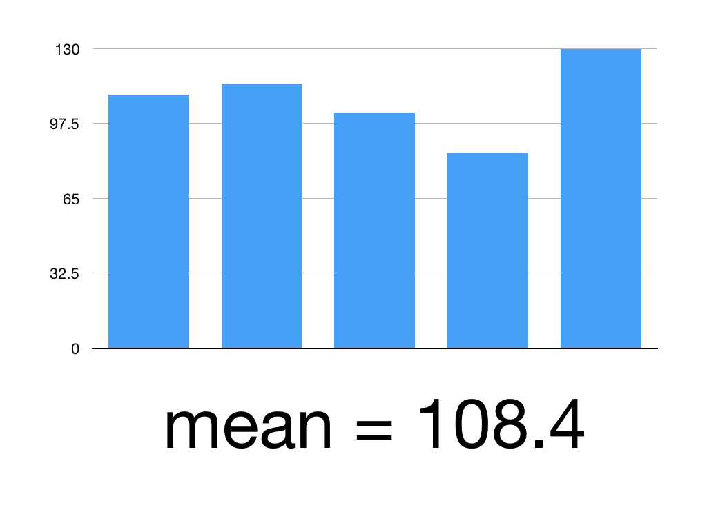
Here are their mean systolic blood pressures:

Patient 1: 110

Patient 2: 115

Patient 3: 102

Patient 4: 85

Patient 5: 130

We want their mean BP within a 95% confidence interval.

First, work out the mean

(110 +115 +102+85+130)/5 = 108.4

Then find the standard deviation = 16.59

That means our SEM is 16.59/square root of 5 = 3.318

The Z value for 95% CI is 1.960

Our mean is 108.4

Our SEM is 3.318

Put it together:

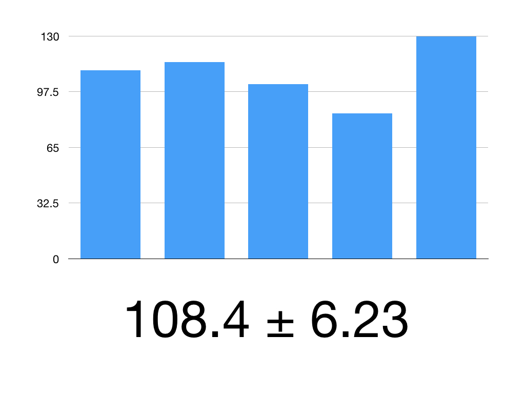
108.4 ± 1.960 x 3.18

1.960 x 3.18 = 6.23

So our 95% CI is 108.4 ± 6.23

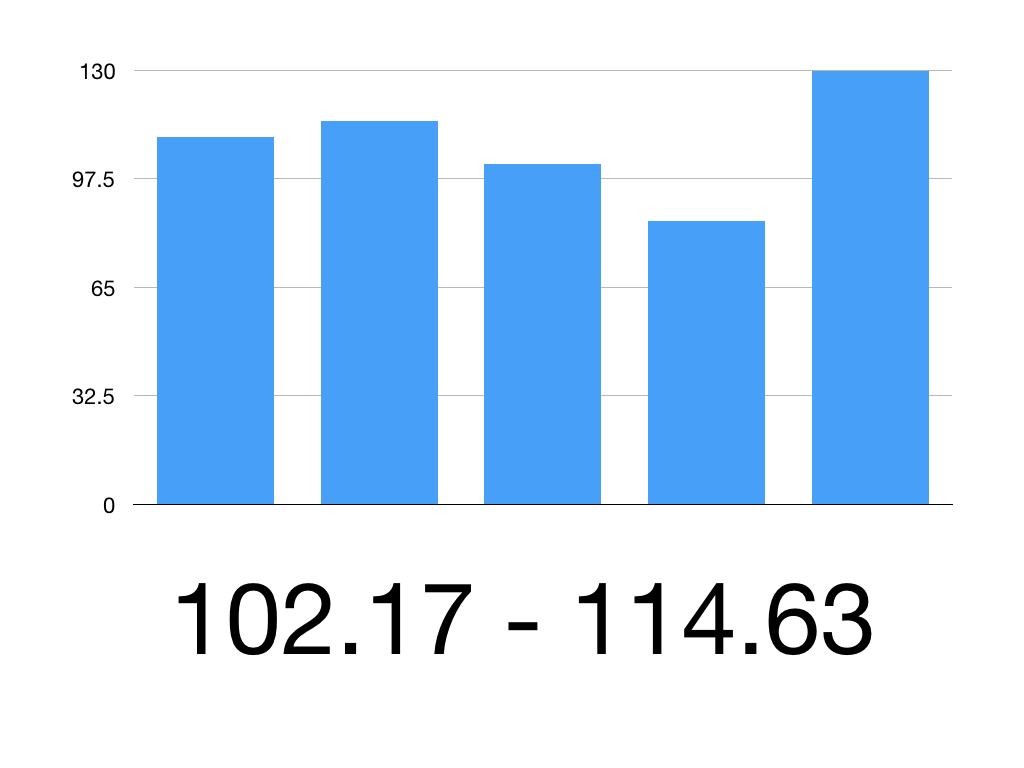
So the 95% CI is 102.17 to 114.63

Therefore we can be 95% confident that the true mean systolic blood pressure is between 102.17mmHg and 114.63mmHg

Outcome measures

Health outcomes involve changes in health status – changes in health of an individual or population, attributable to an intervention. Health Technology Assessment (HTA) is about determining whether an intervention is safe and cost effective.

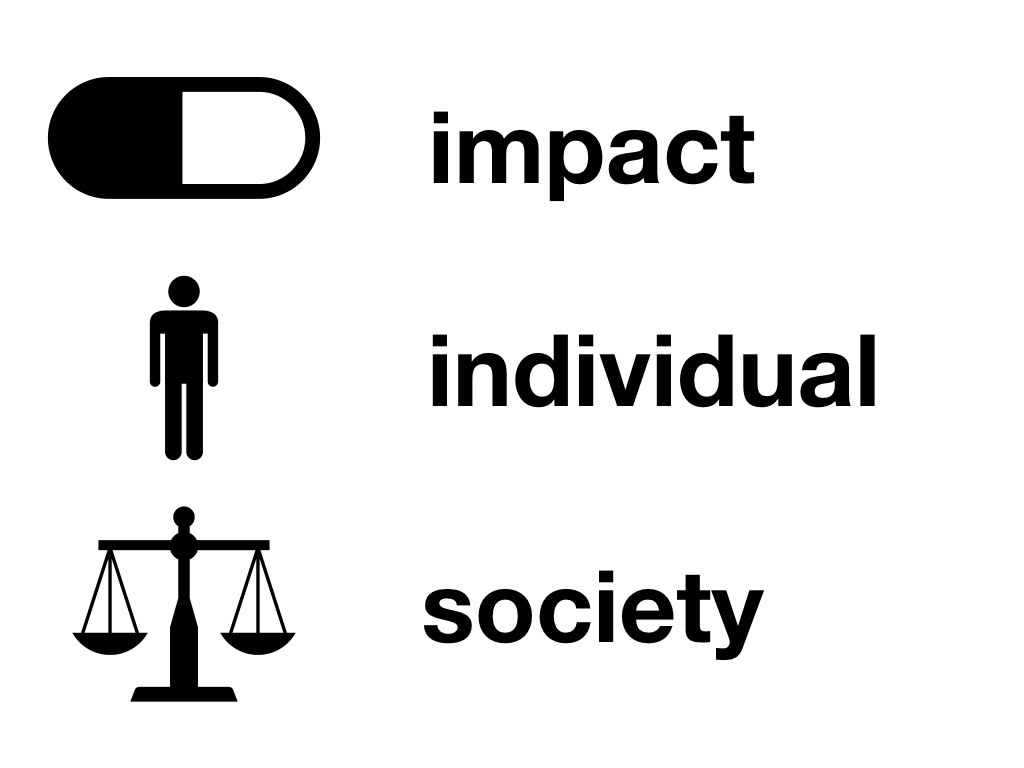
The building blocks of outcome measurement include:
Measurement – What is the impact of the disease? What is the impact of the interventions?
Individual preferences – Trading off length of life for quality of life; what weight is given to different aspects of health
Societal preferences – Relevant to disease or other characteristics

Different scores are used to measure health related quality of life. One often used is the EQ-5D model which was discussed in Session Five. This measures a patient’s quality of life across 5 domains:

Mobility
Self-care
Usual activities
Freedom from pain
Freedom from depression/anxiety

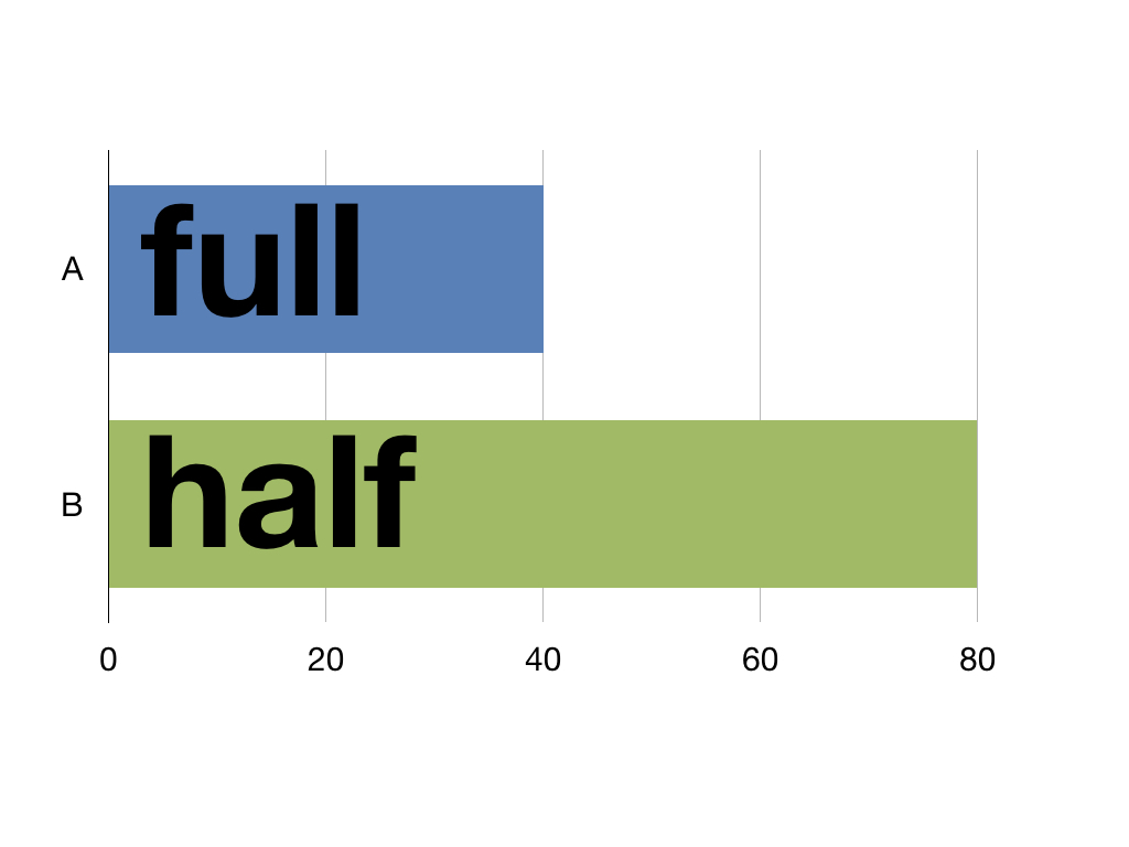
The EQ-5D model is used to calculate Quality Adjusted Life Years (QALYs). These express health outcomes in a way to help policy makers make financial assessments. One year spent in perfect health equals 1 QALY. One year in half perfect health equals half a QALY and so on. This means life isn’t measured in time but in quality as 40 years of perfect health and 80 years of half perfect health are both 40 QALYs.

A decision on funding an intervention can then not just be based on cost but on how many extra QALYs it offers a patient.

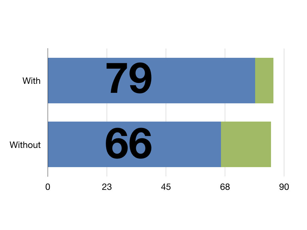
With this pretend intervention patients have an extra 13 QALYs against those without it

For more on Health Outcomes here is a great blog from the BMJ